Statistical methods

This section needs additional citations for verification. Please help improve this article by adding citations to reliable sources. Unsourced material may be challenged and removed. (December 2020) (Learn how and when to remove this template message)

Descriptive statisticsedit

A descriptive statistic (in the count noun sense) is a summary statistic that quantitatively describes or summarizes features of a collection of information, while descriptive statistics in the mass noun sense is the process of using and analyzing those statistics. Descriptive statistics is distinguished from inferential statistics (or inductive statistics), in that descriptive statistics aims to summarize a sample, rather than use the data to learn about the population that the sample of data is thought to represent.

Inferential statisticsedit

Statistical inference is the process of using data analysis to deduce properties of an underlying probability distribution. Inferential statistical analysis infers properties of a population, for example by testing hypotheses and deriving estimates. It is assumed that the observed data set is sampled from a larger population. Inferential statistics can be contrasted with descriptive statistics. Descriptive statistics is solely concerned with properties of the observed data, and it does not rest on the assumption that the data come from a larger population.

Terminology and theory of inferential statisticsedit

Statistics, estimators and pivotal quantitiesedit

Consider independent identically distributed (IID) random variables with a given probability distribution: standard statistical inference and estimation theory defines a random sample as the random vector given by the column vector of these IID variables. The population being examined is described by a probability distribution that may have unknown parameters.

A statistic is a random variable that is a function of the random sample, but not a function of unknown parameters. The probability distribution of the statistic, though, may have unknown parameters.

Consider now a function of the unknown parameter: an estimator is a statistic used to estimate such function. Commonly used estimators include sample mean, unbiased sample variance and sample covariance.

A random variable that is a function of the random sample and of the unknown parameter, but whose probability distribution does not depend on the unknown parameter is called a pivotal quantity or pivot. Widely used pivots include the z-score, the chi square statistic and Student's t-value.

Between two estimators of a given parameter, the one with lower mean squared error is said to be more efficient. Furthermore, an estimator is said to be unbiased if its expected value is equal to the true value of the unknown parameter being estimated, and asymptotically unbiased if its expected value converges at the limit to the true value of such parameter.

Other desirable properties for estimators include: UMVUE estimators that have the lowest variance for all possible values of the parameter to be estimated (this is usually an easier property to verify than efficiency) and consistent estimators which converges in probability to the true value of such parameter.

This still leaves the question of how to obtain estimators in a given situation and carry the computation, several methods have been proposed: the method of moments, the maximum likelihood method, the least squares method and the more recent method of estimating equations.

Null hypothesis and alternative hypothesisedit

Interpretation of statistical information can often involve the development of a null hypothesis which is usually (but not necessarily) that no relationship exists among variables or that no change occurred over time.

The best illustration for a novice is the predicament encountered by a criminal trial. The null hypothesis, H₀, asserts that the defendant is innocent, whereas the alternative hypothesis, H₁, asserts that the defendant is guilty. The indictment comes because of suspicion of the guilt. The H₀ (status quo) stands in opposition to H₁ and is maintained unless H₁ is supported by evidence "beyond a reasonable doubt". However, "failure to reject H₀" in this case does not imply innocence, but merely that the evidence was insufficient to convict. So the jury does not necessarily accept H₀ but fails to reject H₀. While one can not "prove" a null hypothesis, one can test how close it is to being true with a power test, which tests for type II errors.

What statisticians call an alternative hypothesis is simply a hypothesis that contradicts the null hypothesis.

Erroredit

Working from a null hypothesis, two broad categories of error are recognized:

• Type I errors where the null hypothesis is falsely rejected, giving a "false positive".
• Type II errors where the null hypothesis fails to be rejected and an actual difference between populations is missed, giving a "false negative".

Standard deviation refers to the extent to which individual observations in a sample differ from a central value, such as the sample or population mean, while Standard error refers to an estimate of difference between sample mean and population mean.

A statistical error is the amount by which an observation differs from its expected value, a residual is the amount an observation differs from the value the estimator of the expected value assumes on a given sample (also called prediction).

Mean squared error is used for obtaining efficient estimators, a widely used class of estimators. Root mean square error is simply the square root of mean squared error.

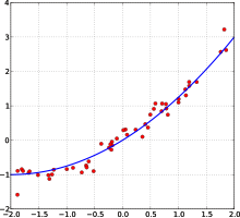
Many statistical methods seek to minimize the residual sum of squares, and these are called "methods of least squares" in contrast to Least absolute deviations. The latter gives equal weight to small and big errors, while the former gives more weight to large errors. Residual sum of squares is also differentiable, which provides a handy property for doing regression. Least squares applied to linear regression is called ordinary least squares method and least squares applied to nonlinear regression is called non-linear least squares. Also in a linear regression model the non deterministic part of the model is called error term, disturbance or more simply noise. Both linear regression and non-linear regression are addressed in polynomial least squares, which also describes the variance in a prediction of the dependent variable (y axis) as a function of the independent variable (x axis) and the deviations (errors, noise, disturbances) from the estimated (fitted) curve.

Measurement processes that generate statistical data are also subject to error. Many of these errors are classified as random (noise) or systematic (bias), but other types of errors (e.g., blunder, such as when an analyst reports incorrect units) can also be important. The presence of missing data or censoring may result in biased estimates and specific techniques have been developed to address these problems.

Interval estimationedit

Most studies only sample part of a population, so results don't fully represent the whole population. Any estimates obtained from the sample only approximate the population value. Confidence intervals allow statisticians to express how closely the sample estimate matches the true value in the whole population. Often they are expressed as 95% confidence intervals. Formally, a 95% confidence interval for a value is a range where, if the sampling and analysis were repeated under the same conditions (yielding a different dataset), the interval would include the true (population) value in 95% of all possible cases. This does not imply that the probability that the true value is in the confidence interval is 95%. From the frequentist perspective, such a claim does not even make sense, as the true value is not a random variable. Either the true value is or is not within the given interval. However, it is true that, before any data are sampled and given a plan for how to construct the confidence interval, the probability is 95% that the yet-to-be-calculated interval will cover the true value: at this point, the limits of the interval are yet-to-be-observed random variables. One approach that does yield an interval that can be interpreted as having a given probability of containing the true value is to use a credible interval from Bayesian statistics: this approach depends on a different way of interpreting what is meant by "probability", that is as a Bayesian probability.

In principle confidence intervals can be symmetrical or asymmetrical. An interval can be asymmetrical because it works as lower or upper bound for a parameter (left-sided interval or right sided interval), but it can also be asymmetrical because the two sided interval is built violating symmetry around the estimate. Sometimes the bounds for a confidence interval are reached asymptotically and these are used to approximate the true bounds.

Significanceedit

Statistics rarely give a simple Yes/No type answer to the question under analysis. Interpretation often comes down to the level of statistical significance applied to the numbers and often refers to the probability of a value accurately rejecting the null hypothesis (sometimes referred to as the p-value).

The standard approach is to test a null hypothesis against an alternative hypothesis. A critical region is the set of values of the estimator that leads to refuting the null hypothesis. The probability of type I error is therefore the probability that the estimator belongs to the critical region given that null hypothesis is true (statistical significance) and the probability of type II error is the probability that the estimator doesn't belong to the critical region given that the alternative hypothesis is true. The statistical power of a test is the probability that it correctly rejects the null hypothesis when the null hypothesis is false.

Referring to statistical significance does not necessarily mean that the overall result is significant in real world terms. For example, in a large study of a drug it may be shown that the drug has a statistically significant but very small beneficial effect, such that the drug is unlikely to help the patient noticeably.

Although in principle the acceptable level of statistical significance may be subject to debate, the significance level is the largest p-value that allows the test to reject the null hypothesis. This test is logically equivalent to saying that the p-value is the probability, assuming the null hypothesis is true, of observing a result at least as extreme as the test statistic. Therefore, the smaller the significance level, the lower the probability of committing type I error.

Some problems are usually associated with this framework (See criticism of hypothesis testing):

• A difference that is highly statistically significant can still be of no practical significance, but it is possible to properly formulate tests to account for this. One response involves going beyond reporting only the significance level to include the p-value when reporting whether a hypothesis is rejected or accepted. The p-value, however, does not indicate the size or importance of the observed effect and can also seem to exaggerate the importance of minor differences in large studies. A better and increasingly common approach is to report confidence intervals. Although these are produced from the same calculations as those of hypothesis tests or p-values, they describe both the size of the effect and the uncertainty surrounding it.
• Fallacy of the transposed conditional, aka prosecutor's fallacy: criticisms arise because the hypothesis testing approach forces one hypothesis (the null hypothesis) to be favored, since what is being evaluated is the probability of the observed result given the null hypothesis and not probability of the null hypothesis given the observed result. An alternative to this approach is offered by Bayesian inference, although it requires establishing a prior probability.
• Rejecting the null hypothesis does not automatically prove the alternative hypothesis.
• As everything in inferential statistics it relies on sample size, and therefore under fat tails p-values may be seriously mis-computed.clarification needed

Examplesedit

Some well-known statistical tests and procedures are:

Exploratory data analysisedit

Exploratory data analysis (EDA) is an approach to analyzing data sets to summarize their main characteristics, often with visual methods. A statistical model can be used or not, but primarily EDA is for seeing what the data can tell us beyond the formal modeling or hypothesis testing task.